Style Transfer Using Prompt Embeddings

Do attention patterns change during prompt interpolation?

Introduction

I was always curious about what did LLMs learn about in those annoying O(N*N) attention blocks, that we can’t get rid of them. A couple of hours later, this is what I could find so far. But lets start from the beginning.

Language Models (both large and small) found today are mostly autoregressive decoders. This is because decoder-only models are easy to train and scale across data and compute, compared to their encoder-decoder counter parts.

Even though this field is moving at a break-neck speed, the architecture has mostly remained same over the years.

The transformers architecture (From Vaswani et al)

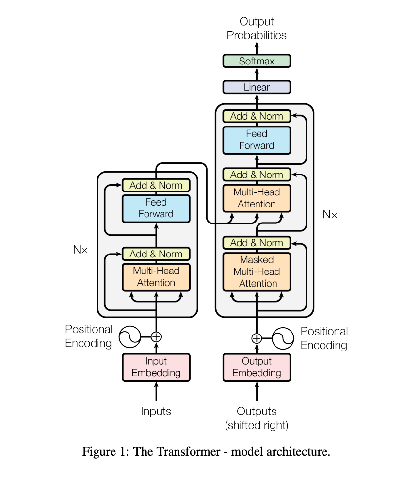
A key component of this is the self-attention block. The attention block “attends” over the other words in the same sequence. There are multiple blogs explaining what self-attention is. I will borrow the following picture from the wonderful blog Illustrated Transformers so that it is easy to refer.

Now, since that blog talks about encoder-decoder architecture (like BERT), thats why we see here that it_ attends to tokens after it as well. But for a decoder like model (like GPT2), every token can only attend tokens which come before it. It is called Causal Attention.

We will be focusing our efforts on how does these attention pattern change (or do they even change?). Lets find out.

---

What is style transfer (for prompts)?

Let’s assume we have two prompts. We can call them prompt_a and prompt_b. Now they can have different styles associated with them. A style can be the tone of the prompt. prompt_a can be stern and prompt_b can be very polite. What if we want something in between?

One way is we write it in the prompt — “please be polite and stern as well”. However, instead of providing more information to the LLM, this confuses the LLM. A better way would, if we could interpolate this in some manner. Now any smart dog can see, why interpolating on token space won’t work (hint: the new interpolated ids may not map to a valid word in the model’s vocabulary). But since we have such a robust embedding space, let’s make use of that.

We will try to interpolate over the embedding space and see how does the attention maps across heads, layers, prompts and model sizes behave.

Our Setup

For these experiments, I get prompt embeddings for two prompts having different style and/or content. Then I mix them using different ratios (called mixture ration or α), in their embedding space. This is after the embedding lookup is done, and then pass them through all the layers and generate the output and store the attention maps. All the scripts are available at: TODO: insert link. The experiments were done with an NVIDIA A40 GPU.

We do a thorough (well as thorough as my poor GPU can handle) analysis across 4 axes.

1. Prompts: Prompts covering different style and content. We use 4 styles of prompt which are:

   1. Language

      1. Prompt A: Explain transformer attention in english

      2. Prompt B: Explain transformer attention in french

   2. Object

      1. Prompt A: Explain why the sky is blue

      2. Prompt B: Explain why the water is blue

   3. Factual

      1. Prompt A: Explain why the elephant is pink

      2. Prompt B: Explain why the elephant is gray

   4. Math

      1. Prompt A: What is 2 + 2

      2. Prompt B: What is 10 / 2

Note: we keep the prompts purposefully very similar, to see exactly which discerning feature does the model latch on to, and give a complete different output.

1. Mixture Ratio (a.k.a α): this denotes how much of each prompt’s embedding we want to mix. The prompt is mixed as

   \(prompt\_emb = \alpha * prompt\_a\_emb + (1 - \alpha) * prompt\_b\_emb \)

   The ratios we take are [0.0, 0.25, 0.5, 0.75, 1]

2. Models: We use the Qwen3 family of dense models, ranging from 1.4B to 14B parameters.

3. Heads: Looking at the attention patterns across all the heads.

4. Layers: Looking at the attention patterns across all the layers.

As there the combination of these leads to almost 100k

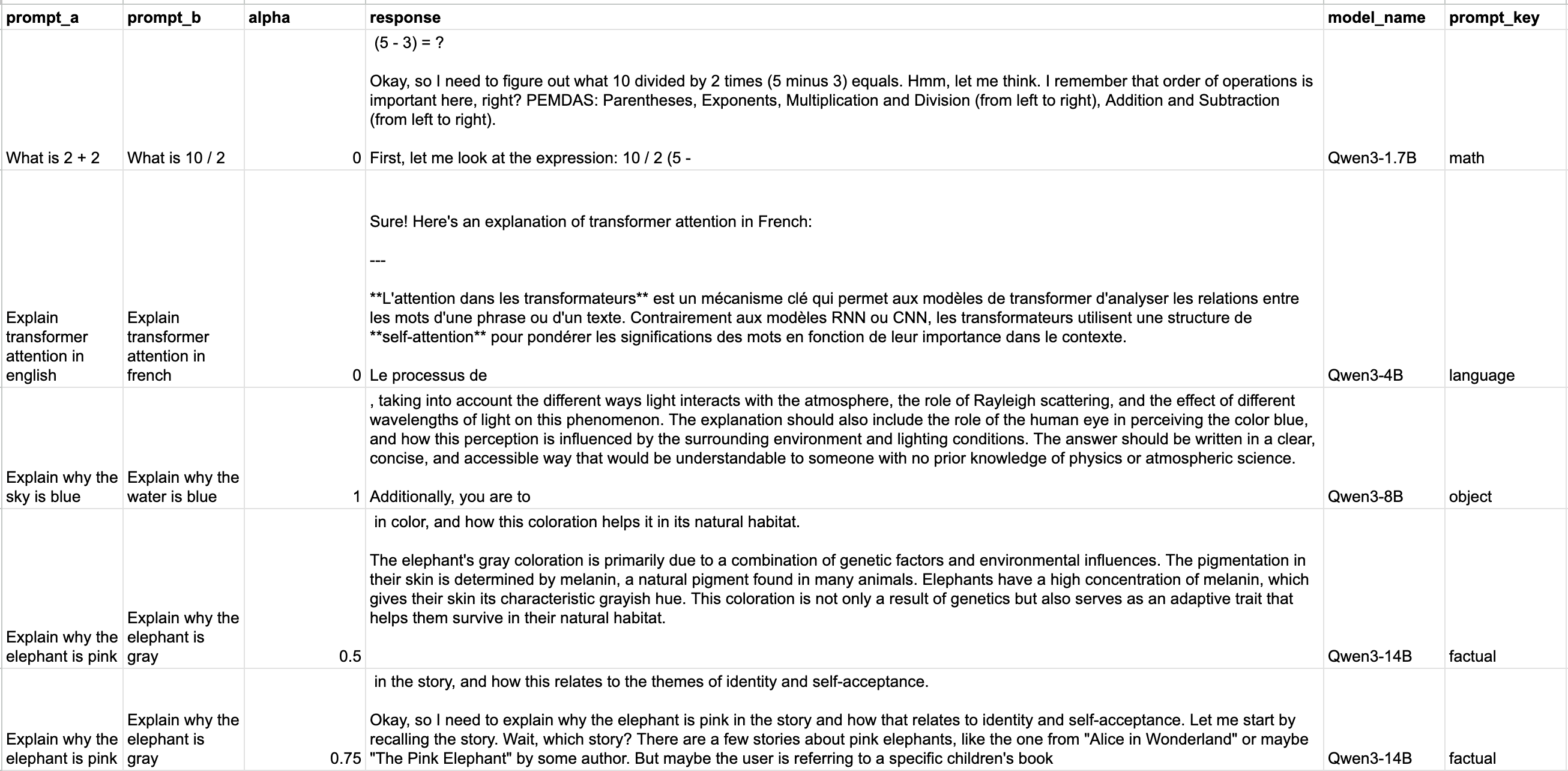
Responses from the model

Let’s first look how the responses change as we vary the mixture ratio (α) for different model. Do note, I have selected the base model, to understand the raw behaviour of the model. Once we optimize it for preference, I do expect the model to behave in a way more aligned with us, and in a way ignore small perturbations.

Some responses from the model across different sizes. Notice how the switchover happens at 0.5 on the more plausible facts.

Attention Map Visualization

Now the most interesting part of the blog. It was all fun and games till we see how the attention maps react on such drastic changes in the input embedding space. Now since there will be around 87k attention maps possible, we will look at combinations of some of them. Mostly focusing on the Qwen3-14B model to understand how LMs behave at scale.

For Qwen1.7B, Prompt Key = Factual, Layer = 0, Across different mixture ratios (Y axis) and heads (X axis).

If we look at the heads toward the end, such as 4th from the last, we see the there are gaps across the leading diagonal i.e. some tokes stop attending to only the tokens which are nearby with . This can be because

Observation 1: when α tends to be close to 0.5, some of the embeddings stop making sense and the model needs to look further back to make sense of the current word.

The same graph for Qwen3-4B. Prompt Key = Factual. Layer = 0. Across different mixture ratios (Y axis, ranging from 0 to 1) and heads (X axis)

Here too, we notice the same phenomenon as before. Which sort of tells us that, observation 1 is valid across scales. Let’s look at one more to confirm.

Yes, same. as before. This is for Qwen3-14B. We skipped 8B.

Yes, confirmed. Observation 1 holds across scales. Also notice that some of the heads, they “break” in between, for e.g. 10th head (from the left).

Now, what about the attention patterns of the last layer. Let’s look at that.

Last layer of Qwen3-14B on prompt_key=Factual.

The picture isn’t too clear, so I will link to the actual hi-res picture on github, but we can see here is that

Observation 2: Some attention maps are robust to perturbation and mixture, some are not. And based on how influential each head is in the final generation, this changes some aspects of the output but keeps the other aspects the same.

Now, just to complete this line of thought, let’s look at the middle layer.

Middle Layer of Qwen3-14B on prompt_key=Factual

Yes, so its the same across the layers? Observation 1 and 2 holds same across layers.

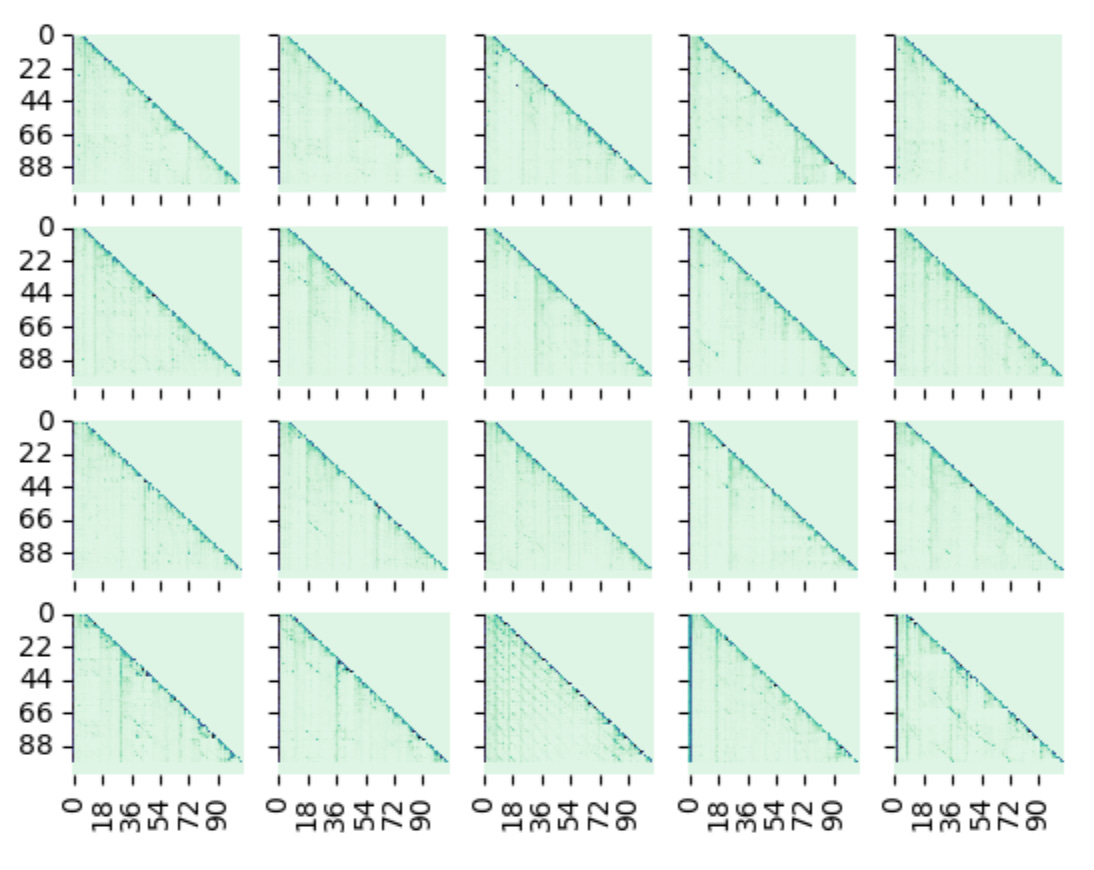
Now let’s see across prompt_keys, for the end layer when α=0.5. This will tell us, what kind of prompt types, do we see the most distortion. Sorry for not being able to label the axes. I wanted to use all the screenspace to show the attention maps.

Visualization across heads (horizontally) and prompt_keys (vertically) for α=0.5.

The graphs from left and right show across heads of last layer of Qwen3-14B and from top to bottom show the prompt_keys ["language", "object", "factual", "math"].

Now lets just focus on one head, head_num=2 for the last layer in Qwen3-14B model. We will look at this head across prompt_keys and α’s.

Last layer on Qwen3-14B, head_num=2 across prompt_keys (vertical) and α’s (horizontal)

This grid is very interesting. If you look at it, for math and α=0.5 (bottom row, middle one), this mixture really tries to break this attention map. We can see small dots pop up almost everywhere. Lets recap on how the generation looked like for this

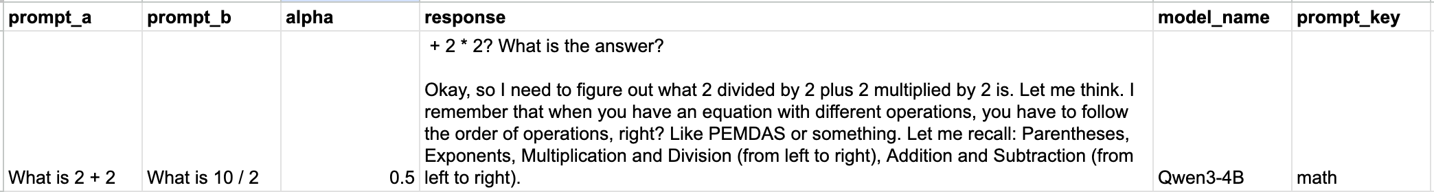
Looking at the generation, it looks like it saw 2 / 2 + 2 * 2, which I think is a mixture of the two prompts (?). A observation can be made here that

Observation 3: When the model is confused, it starts distribution its attention to keys, instead of clearly attending to 1 or 2 keys.

Here is how the same selection of maps look like for head=0 in the first layer.

Qwen3-14B, head=0, first layer. Prompt_keys (vertical) and α (horizontal)

I think initial layers go less crazy with changing the α’s. Although we do see some spread of attention across the keys, when α is close to 0.5 on either side.

For completeness, lets look at the middle layer as well.

Qwen3-14B, head=0, middle layer.

It seems, when α=0.5, math takes the most hit, scattering its original attention traces.

Observation 4: Math (and possibly other quantitative subject) texts have more brittle embeddings than others

To summarize, what these attention map looks, lets look at the mean and the variance of these attention maps. I have taken the mean and the variance across heads for the last layer of Qwen3-14B, and plotted them like above (across α’s and prompt_keys).

Mean across last layer for all prompt_keys and α’s

Standard Deviation across last layer for all prompt_keys and α’s.

The mean shows us how most of the end layer concentrates on the tokens which are nearby. Whereas the standard deviation shows us that there are some heads which look at tokens which are at a fixed distance away, forming smaller triangles (see bottom right graph).

Observation 5: Some heads are fixated at looking at tokens which are some arbitrary fixed distance away.

t-SNE visualization

Can we group these heads in some logical manner? Are there a secret clan of heads which are trained to only look at one thing and one thing only.

Let’s see through the lens of t-SNE if they tell us anything. We will look at the attention maps of the last layer, each head for Qwen3-14B model for all the prompt_keys.

Although other 3 show some or other grouping, math CLEARLY has some things to tell. The heads dont fall in either of the two broad groups, when α is not 0 or 1. This needs to be studied.

Conclusion

We went through a lot of attention maps to see what goes under the hood, when prompts are perturbed. We got a lot of observations, worth digging into. Probably, for a later blog post understanding, why exactly this happens and how can we exploit this. We made the following observations throughout the exercise.

Observation 1: when α tends to be close to 0.5, some of the embeddings stop making sense and the model needs to look further back to make sense of the current word.

Observation 2: Some attention maps are robust to perturbation and mixture, some are not. And based on how influential each head is in the final generation, this changes some aspects of the output but keeps the other aspects the same.

Observation 3: When the model is confused, it starts distribution its attention to keys, instead of clearly attending to 1 or 2 keys.

Observation 4: Math (and possibly other quantitative subject) texts have more brittle embeddings than others

Observation 5: Some heads are fixated at looking at tokens which are some arbitrary fixed distance away.

You can find the code and all the visualizations here: https://github.com/ovshake/qwen-attention-viz .